

Input data
Table 2 summarizes the input data used in the 3D geological and 3D hydrological model-building workflow described in this study. It compiles information on hydrofacies interfaces, including surface topography, bathymetry, hydrogeological units, fault systems, and overland flow parameters, as well as the URL where the data can be found and their references.
Table 2 Type, Name, References, URLs, characteristics, and format for the input data used in the construction and verification of the 3D geological and hydrogeological models; all URLs were last accessed in June 2025.Digital Elevation Model (DEM)
To define the top of the modeled domain, a sufficiently well-resolved DEM was required. Surface topography was represented using the ASTER Global Digital Elevation Model (GDEM Version 383), which offers a spatial resolution of 1 arc-second (approximately 30 m). For the submarine topography in the Suruga Bay area, bathymetric data from the GEBCO_2024 (General Bathymetric Chart of the Oceans84 were merged with the land DEM. In addition, lake bathymetry data provided by the Geospatial Information Authority of Japan85 were appended to accurately represent lake bottoms within the study area. A similar but global product, the GLOBathy dataset86, is also available and offers comparable bathymetric information.
Hydrological network
To accurately represent surface water features in the hydrological cycle, geographic information from the national river and lake maps was used87,88. The datasets include river centrelines and lake surface areas across all of the Japanese archipelago, based on a 1:25,000 scale. The coarser, global HydroRIVERS89 and HydroLAKES90 datasets could be considered as alternative data sources with global coverage where more highly resolved local datasets are unavailable.
The current integrated hydrological model implementation focuses on the natural hydrological system, excluding anthropogenic modifications such as dams, streamflow regulation structures, and municipal irrigation networks. This approach allows for a clearer baseline understanding of natural hydrodynamics within the catchment.
Hydrofacies boundary surfaces
As a basis for the construction of the highly resolved, catchment-scale hydrofacies used in this study, existing information from the NHM (500 m x 500 m horizontal resolution78 was used. The digitized hydrofacies information as implemented in the NHM was obtained directly from GETC and supplied as shapefiles, containing contour lines of the bottom bounding surface of each hydrofacies as well as polygons defining their horizontal extent. These shapefiles are provided in the data repository associated with this paper91.
While the existing hydrofacies product of the NHM includes estimated surfaces of all major hydrofacies of Mt. Fuji catchment, the model was not designed to be consistent at the sub-catchment or local scale, and as a result, some surfaces were absent or discontinuous in certain areas of the catchment, or defined too coarsely to match the detailed geological structures relevant at the sub-catchment scale. To produce hydrologically robust simulations of Mt. Fuji catchment, additional data were thus needed to: (i) complete the near surface hydrostratigraphy across most areas, (ii) complete and fill internal gaps in the existing hydrofacies using current geological information to ensure full spatial coverage, and (iii) improve resolution in geologically complex areas.
The following information sources and input data were thus considered: surface (i.e. outcrop) information from the geological map of Fuji Volcano, hydrogeological layers’ bottom elevation contours from localized studies around the catchment, and borehole logs and geological cross-sections from both geological and hydrogeological studies on Mt. Fuji.
It is important to note that in the case of the Mt. Fuji catchment, a preliminary hydrofacies surface dataset was available and served as the foundation for the workflow presented here. In regions where such datasets are not available, equivalent hydrofacies surfaces can be constructed from geological cross-sections, borehole records, and other stratigraphic information by following the same workflow outlined in this study.
Faults
Data for the Fujikawa-Kako Fault Zone were obtained from the Active Fault Database of Japan64. Information on faults is essential not only for accurately modeling the geological structure, but also for assigning hydrogeological parameters and understanding flow discontinuities or barriers in hydrological models. Although the FKFZ comprises numerous conjugate faults, for modeling purposes this study simplified the system to two major fault traces. The fault system is about 30 km long and oriented towards the North with a 10° angle towards the East. Given likely variations along the fault zone, both traces were conceptualized as predominantly vertical structures, consistent with previous studies65,75.
A significant contrast in aquifer thickness was observed across the FKFZ: aquifers on the eastern side reach depths of up to 300 meters, while those on the western side are generally limited to around 100 meters.
Land-use and land-cover
To accurately parameterize overland flow in the integrated hydrological model, land-use and land-cover (LULC) data were used. This information was obtained from the 2022 High-Resolution Land-Use and Land-Cover Map of Japan (v23.12), developed by JAXA’s Earth Observation Research Center (EORC)92. This dataset includes 14 land-cover categories, which are later grouped into 5 hydrologically relevant categories.
SoftwareGeographic information system
A geographic information system (GIS) software was used to pre-process and post-process the model’s input and output files. In other words, it was used to convert data into the formats required by geological and integrated hydrological modeling and visualization tools, as well as to present some of the results. In this study, the free and open-source QGIS platform (QGIS Association; version 3.38.2; https://www.qgis.org) was used. Alternatively, the commercial software ArcGIS Pro (ESRI; https://www.esri.com) could also be used.
Geological modeling software
A 3D geological modeling software was used to create detailed representations of subsurface structures by integrating various geological data, and to visualize complex geology and supports analysis and simulations. Here, we chose the commercial software Aspen SKUA (Aspen Technology Inc.; SKUA-GOCAD Paradigm 19; https://www.aspentech.com/en/products/sse/aspen-skua). Alternatively, the free and open-source GemPy software93 (https://www.gempy.org) could be used.
Numerical mesh generation software
A numerical mesh generation software was required for the generation of a triangular finite element mesh. For the simulation of geologically and hydrologically complex systems such as volcanic island aquifers, and specifically Mt. Fuji watershed, a powerful mesh generation software capable of producing unstructured meshes for numerically efficient and robust calculation was needed. The numerical mesh generation software must be able to adapt the numerical mesh to a relatively large number of geological, hydrological, and topographical features of the system that are simulated, which can be hydrofacies outlines, geological faults, water body outlines, steep slopes, areas of different land cover and land use, as well as water use infrastructure such as pumps and drains. This approach ensured that important hydrological features were well represented while minimizing the total number of computational nodes.
In this study, we used the commercial mesh generator AlgoMesh (HydroAlgorithmics Pty Ltd; version 2.0.20.32621; https://www.hydroalgorithmics.com/software/algomesh), which generates high-quality grids for multiple finite-volume and finite-element simulation software. Alternatively, the open-source 3D finite element grid generator Gmsh94,95 (http://gmsh.info) could be used.
Integrated surface-subsurface hydrological modeling software
An Integrated Surface-Subsurface Hydrological Modeling (ISSHM) software was required for simulating the full water cycle—capturing interactions between rainfall, surface runoff, infiltration, and groundwater flow—to support accurate water resource management and impact assessments under changing climate conditions. One of ISSHM’s core strengths is their ability to explicitly simulate the interactions between surface water and groundwater with spatially heterogeneous parameters, which is critical for adequately representing hydrological processes in complex geological settings such as alpine catchments and volcanic islands6,96. Another key advantage of ISSHMs is their ability to explicitly simulate solute transport throughout the surface and subsurface, as well as across their interface, which enables advanced model calibration and deeper interpretation of environmental tracer data across multiple sources10,97,98,99,100,101,102,103,104,105. These capabilities make ISSHMs particularly valuable for predictive modeling, especially when evaluating the effects of climate change on groundwater systems106,107,108. However, it should be noted that the current model resolution, designed to balance geological detail with computational feasibility, may limit its immediate suitability for explicit solute transport simulations. Users aiming to apply the model for such purposes should consider refining the mesh or adapting the model structure accordingly. Alternatively, simplified transport analyses can be readily achieved with the current model structure using a particle tracking approach, which relies exclusively on the advective flow field109.
In this study, we used the research-oriented commercial software HydroGeoSphere (HGS) (Aquanty Inc.; revision 2817; https://www.aquanty.com). In HGS, surface and subsurface flow as well as heat and mass transport are simulated in a fully integrated manner under consideration of 2D surface flow, variably saturated subsurface flow, discrete fracture flow, vegetation-land-water interactions, density-dependent flow and transport, as well as winter hydrological processes – all processes which are relevant for the studied site97,98,100,110,111,112. Alternatively, the open-source software ParFlow113,114 (https://parflow.org) could be used.
Computational fluid dynamics, visualization and processing software
A visualization and processing software was required to interpret, analyze, present and communicate the results of hydrological simulations in a clear and accessible way. These tools allow users to process large and complex datasets, create detailed plots and extract meaningful patterns from spatial and temporal model outputs.
Here, Tecplot 360 (Tecplot, Inc.; version: 2024.R1; https://tecplot.com), a powerful commercial software for 3D visualization, and post-processing, of large numerical models was used. Tecplot is the recommended visualization and postprocessing tool for HGS, enabling efficient exploration of simulation results, including groundwater flow paths, concentration fields, and time-series data. Alternatively, the open-source, multi-platform data analysis and visualization application ParaView (https://www.paraview.org) can be used.
Workflow
Figure 2 illustrates the workflow for developing a 3D geological model and a 3D integrated surface-subsurface hydrological model in geologically complex volcanic watersheds. The process, which is presented in detail in the sections below, started with the collection, organization, and preprocessing of all available geological and hydrofacies data using a GIS software. In parallel to the input data pre-processing, a numerical mesh was generated and optimized using a numerical mesh generation software. In the next step, this data was imported into a 3D geological modeling software, where stratigraphic units, faults, and hydrofacies boundaries were interpreted and assembled into a geologically coherent 3D model. Modeled hydrofacies boundaries were then exported back to the GIS software for rasterization. Finally, the rasterized hydrofacies, numerical mesh, and hydraulic input data (such as flow boundary conditions and parameters) were integrated into the hydrological model. Flow properties, as well as initial and boundary conditions were assigned to the subsurface and surface domains, and the simulations were controlled by a set of running parameters to produce a catchment-scale integrated surface-subsurface hydrological model of Mt. Fuji watershed. The resulting outputs were then visualized and reviewed for validation by comparing them with observations.
Fig. 2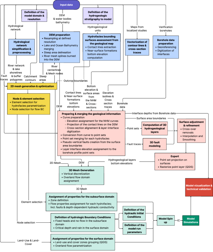
Workflow for developing an integrated surface–subsurface hydrological model in geologically complex volcanic watersheds. Each colored box corresponds to a major process described in the main text: conceptualization (purple), input data processing (blue), 3D geological modeling (pink), numerical mesh generation (yellow), 3D integrated hydrological modeling (green). Data transferred between steps is indicated along the connecting arrows.
ConceptualizationDefinition of the model domain and resolution
The surface model domain, representing the Mt. Fuji catchment, was delineated to represent the topographic catchment using the “catchment” tool in QGIS. The resulting catchment area spans approximately 1,650 km². Vertically, the model extends from 3,776 m asl, corresponding to the summit of Mt. Fuji, to −1,100 m asl, representing the bottom of the Neogene Fujikawa, Nishiyatsushiro, and Tanzawa groups, that is, the bottom of Mt Fuji’s basement (BS). The model was vertically cut at the shoreline of the Suruga Bay.
The optimal model resolution depends heavily on the resolution, distribution and quality of the base data sets. In the case of Mt. Fuji, the data sets (i.e. geological map and NHM) used to create the hydrogeological framework form the upper limit for the model resolution. For example, the geological map of Mt. Fuji59 with a resolution of 1:50,000 shows geological details of 50 m in diameter at this map scale, with a size of 1 mm. A finer resolution, therefore, would not add geological accuracy and could lead to misleading model detail.
From a numerical stability perspective, there is a trade-off between a fine mesh that may create unfeasibly long runtimes due to the many discrete points to calculate, and a coarse mesh, which may result in numerical instability due to the resolution being too low to resolve the physical behavior that is simulated. Considering the large spatial extent of the model domain, a horizontal resolution of 75 m was selected to strike a balance between sufficient spatial detail, numerical stability, and acceptable computational performance (i.e., simulations finishing within hours to days).
Definition of the hydrogeologic stratigraphy to be modeled
The hydrogeological stratigraphy of Mt. Fuji catchment is based on the hydrofacies classification presented in Table 1.
Input data processing
In the geological modeling software used in this study, the base elevation of each hydrofacies must be imported as a vector dataset (.shp) to allow construction of a 3D model. As a result, all spatial datasets must be preprocessed and formatted within a GIS software before import. A critical step in this process is ensuring that all geospatial data share a consistent coordinate reference system to maintain spatial accuracy during model construction.
Hydrological network simplification and preprocessing
The base hydrological network dataset includes all rivers, streams, and detailed lake shorelines. However, incorporating the full-resolution dataset into the numerical mesh would result in excessive refinement and prohibitively high computational costs. To address this, the data were preprocessed in QGIS. Only the main river segments (stream orders 1 and 2) were retained, and both river and lake shoreline geometries were simplified using the “Simplify” tool to reduce vertex density while preserving essential hydrological features. These simplified line features were then exported to the meshing software and used to guide local mesh refinement. Additionally, buffer polygons were generated 100 m around the selected river segments and lake shorelines to further control the mesh element size during mesh optimization.
DEM preparation
The surface topography and bathymetry of lakes and coastal areas define the top boundary of the model. As in the raw DEM, elevation values over water bodies correspond to the free surface water level; the Fuji Five Lakes were merged with the DEM to accurately represent submerged terrain. To match the DEM to the model resolution, the merged 30 m DEM raster was upscaled to a horizontal resolution of 75 m using the “SAGA resampling” tool in QGIS, applying mean-value aggregation.
As necessary for all physically based surface water flow modeling, the DEM had to be further refined in parallel to the mesh generation in order to ensure consistency between DEM coarsening and mesh refinement115. Specifically, river centerlines generated in the 2D mesh had to be reconsidered in the DEM to prevent artificial blocking of surface water flow along the stream network, which would be caused by DEM simplification linked to the mesh’s coarseness at this spatial scale. This was achieved by stream-burning using the r.carve tool from the GRASS toolbox in QGIS. Parameters included a 100 m channel width, a 2 m channel depth, and the exclusion of flat flow paths to preserve hydrological connectivity.
To further support mesh refinement in terrain where significant hydraulic gradients are expected, a set of polygons encompassing all areas with slopes greater than 20% was generated.
Finally, a regular point grid (.shp) with 75 m spacing was created in QGIS, centered on raster pixels, and used to sample elevation values from the DEM. This point dataset was then exported to Aspen SKUA for geological modeling.
Hydrofacies bounding surfaces assessment from the geological map
The geological map of Mt. Fuji provides polygon vector data of the outcropping geology across the entire catchment. To incorporate this information into ISSHM modeling, the original map—comprising numerous geological units—was first simplified by grouping formations into relevant hydrofacies (Fig. 1c) and merging them into a single polygon shapefile for each hydrological unit. To estimate the base elevation of each hydrofacies, the following principle was applied: where a formation is in contact with an older unit, the surface trace of the boundary between the formations represents the base of the younger formation. Therefore, the relevant contact lines were extracted as vector shapefiles and exported to the geological 3D modeling software.
Additionally, the surficial hydrofacies AL and MF were largely absent from the coarse NHM despite their dominance in the outcropping geology across much of the catchment. In agreement with the information available from the NHM and with localized modeling studies31,116, a linearly increasing thickness from 0 m at the summit of the volcano to 10 m for AL and 20 m for MF at a radial distance of 12 km from the summit, i.e., the center of the plains around Mt. Fuji, was assumed. To incorporate this assumption into the 3D geological model, a regularly spaced point grid was generated in QGIS, and surface elevation values were extracted from the DEM. A spatial linear function was then applied at each point to estimate the bottom elevations of AL and MF based on terrain elevation. The resulting dataset was clipped to include only areas where AL and MF were present according to the geological map, assuming that MF underlies AL wherever AL is present.
Vectorization of the contour lines and cross-sections
Some local studies provided information about the bottom elevation of hydrofacies in the form of contour maps or (hydro)geological cross-sections (Table 2). To use this information in the 3D geological modeling, the contour lines and cross-sections needed to be vectorized in QGIS. First, the maps are georeferenced to the chosen Coordinate Reference System (CRS). The isolines of the bottom elevation of each hydrofacies are then manually captured in a vector file, with the elevation of each line reported as an attribute. For the cross-sections, the traces are manually captured as lines in a vector file.
Borehole data preparation for the model verification: georeferencing and digitization of layer interfaces
For geological model verification, borehole data from some geographically localized studies were used (Table 2). For this purpose, borehole locations must be compiled into a point vector layer. Subsequently, the borehole logs are interpreted to identify the depth of each of the hydrofacies present in a log, and these points are then added as an attribute to each respective borehole point in the vector layer.
3D geological modeling
All processes in the geological modeling software Aspen SKUA, including data import and processing, are performed manually to enable greater control and customization during model construction.
Importing the data
Point and line vector layers were imported into Aspen SKUA as “cultural data”. To maintain organization within the project, these inputs were grouped into feature categories corresponding to each hydrofacies.
The DEM and borehole location point sets, isolines representing the surface bottom elevations and areas from the NHM, and fault traces were imported directly from vector files. Cross-section images, trimmed to their geological boundaries, were imported as 2D voxets. Additional vector line data — including contact lines and bottom elevation of near-surface formations from the geological map, isolines from localized geological studies, and cross-section traces prepared in QGIS — were also imported for further processing. Note that in Aspen SKUA, imported line vector layers are referred to as “curve sets”.
Preparing and merging the geological information
For the isolines from the NHM, the script editor tool in Aspen SKUA was used to assign elevation values as curve properties. The contact lines from the geological map were vertically projected onto the DEM. For the cross-sections, the imported voxets were resized using control points by selecting the trace edges and manually adjusting their elevation based on the DEM and the depth indicated in the cross-section. Once correctly aligned, a new 3D curve was digitized by placing segments along the image to trace the bottom elevation of each hydrofacies.
All resulting curves were then converted into point sets. For each hydrofacies, a single merged point set was created by combining all relevant inputs. The only exception is for layers displaced by the FKFZ faults — specifically BS, OLF, and OLFM — for which two separate point sets were created to represent the east and west sides of the fault zone.
The curves defining the surface area boundaries from the NHM were used to generate pseudo-vertical faults. These extended well beyond the vertical limits of the model domain and were used to clip the hydrofacies surfaces in a later step.
Finally, a separate point set was created for each of the MF, FV, and OLFM layers, whose interfaces were also recorded in borehole profiles. As with the isolines, elevation values were assigned using the script editor tool based on the attribute tables of the imported points. These data were used solely for technical validation of the model and were not included in the actual model computations.
Computation of 3D hydrofacies layers
The bottom surfaces of the hydrofacies layers were computed explicitly through direct triangulation of these point sets. This method enables manual adjustments based on geological interpretation, which is especially valuable in geologically complex regions. Unlike implicit modeling, which relies on algorithm-driven interpolation and includes statistical uncertainty estimation, this explicit approach offers greater transparency and control.
3D fault modeling
Fault traces were used to construct vertical fault surfaces in Aspen SKUA using the software’s dedicated fault modeling tool. Each fault was represented as a single-element vertical surface extending continuously through all geological layers, ensuring structural consistency across the model.
Surface adjustment and refinement
After computing the geological surfaces, crossing surfaces were corrected in accordance with the stratigraphic sequence, where more recent geological layers overrule older layers. A key constraint in the modeling process is that no layer can exist above the outcrop of its preceding units. To enforce this, the surfaces were trimmed using the outcropping extents of the lower layers—implemented in Aspen SKUA by cutting one surface with another.
The surface area boundaries from the NHM were treated as minimum extents, allowing for the possibility that layers, where warranted by the other available data, extended beyond them. The final horizontal extent of each layer was determined based on the distribution of outcropping formations.
Respecting the mapped outcrops and contact lines proved especially challenging in the fault zone, where layers had been displaced or eroded. Manual adjustments were made to maintain the correct stratigraphic relationships while honoring mapped surface geology. Where needed, interpolation was used to smooth out numerical artifacts. Finally, surface smoothing and decimation were applied to simplify layer boundaries, using a vertical tolerance of 1 meter. Figure 3 presents the final geological model constructed in Aspen SKUA.
Fig. 3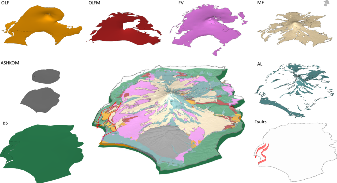
3D geological model snapshot, taken in Aspen SKUA, with a factor two of vertical exaggeration. The layers are the bottom elevation of each hydrofacies: BS (forest green), ASHKOM (grey), OLF (orange), OLFM (dark red), FV (pink), MF (gold), AL (blue). The fault traces and surfaces are depicted in red.
Export
Once a 3D geological model is finalized in Aspen SKUA, it needs to be exported in a format compatible with the selected hydrological simulation software. Here, we used the finite element ISSHM HGS, which requires hydrogeological layer interfaces (i.e., hydrofacies surfaces) to be provided as raster files. A key consideration during export is ensuring sufficient spatial resolution to accurately represent complex geological features, such as fault zones. To satisfy this requirement, we used a regular point grid with a horizontal resolution of 75 meters—the same grid originally created for exporting the DEM from QGIS to Aspen SKUA. Elevation values for each layer were assigned using a vertical projection method, starting from the DEM and progressing downward through the stratigraphy. In areas where a geological unit was absent, its volume was artificially “closed” by the bottom of the overlying hydrofacies, ensuring that each layer spans the entire horizontal model extent, as required by finite element models like HGS. The processed point grid was then re-exported to QGIS, where it was interpolated into raster format (TIN interpolation tool with 100 m resolution) for input into the HGS modeling workflow.
Numerical mesh generation
To construct a comprehensive 3D model of the entire catchment within a hydrological simulator, the first step is to generate a 2D numerical mesh. This mesh discretizes the horizontal extent of the simulation domain at a resolution that balances spatial accuracy and computational efficiency while incorporating constraints from geology, hydrology, topography, land use/cover, and water infrastructure. In the second step, a 3D mesh is built by expanding the 2D mesh vertically using the interface elevations of the various hydrofacies layers.
Horizontal mesh generation and optimization
Although HGS supports both finite element and finite difference methods, the present model was developed using the finite element approach. Accordingly, mesh generation was carried out with the finite element mesh generation software AlgoMesh using line and polygon vector files as input. The catchment contours, resampled at a 400 m resolution, define the outer extent of the mesh. Simplified river centerlines, lake shores, and fault traces were also resampled at 400 m resolution and incorporated into the mesh.
To guide mesh refinement during optimization, steep-slope zones and buffer polygons around the hydrological network were used to apply spatially variable constraints on maximum edge length. These were set to 200 m near rivers and fault traces, 250 m along lake shores, and 500 m in steep-slope areas. The maximum edge length across the rest of the domain was set to 750 m.
The final refined 2D finite element mesh, which contains 24,800 nodes and 49,044 triangular elements, with nodal spacing ranging from 185 to 750 m, was then exported in the AlgoMesh-HGS interchange format A2H, which is based on standard ASCII mesh file structures. River centerlines and mesh nodes were also exported as vector data for subsequent use in DEM preprocessing.
While ideally, the mesh would also be refined using the outcropping boundaries of geological layers to better align surface elements with mapped formations, this was omitted here to avoid excessive refinement, given the complexity of the geological map. Doing so would have significantly increased computational costs.
Node and element selection
During the ISSHM model setup, initial parameter values representing the system’s physical properties were assigned to nodes and elements of the finite element mesh. Therefore, geological and hydrological features were spatially mapped to the mesh in AlgoMesh, utilizing line and polygon shapes generated in QGIS, which enables the targeted selection of relevant nodes and elements.
Flow boundary conditions were applied to specific node sets located along the model boundaries, notably along the Suruga Bay coastline, the catchment perimeter, and river outflow points. Hydrofacies were parameterized by using the polygon element selections and expanding these in the vertical dimension to enclose all numerical model layers over which the respective hydrofacies were assumed to exist. Elements adjacent to the fault lines were also selected for the hydrogeological parametrization.
All node and element selections were exported from AlgoMesh in HGS-compatible formats (.nchos for nodes and.echos for elements).
Integrated hydrological modeling3D mesh generation
In order to preserve fine-scale surface features such as riverbeds and prevent the formation of artificial depressions or sinks, the elevation of the surface layer of the model was defined by directly mapping the elevation values from the fully processed DEM (which includes lake and coastal bathymetry as well as burned streams) at each given node location to that respective node by importing the 2D finite element node locations and using the raster value extraction tool in QGIS.
Elevations of the hydrofacies interfaces were defined by first generating layers for each hydrofacies bottom in HGS using the “generate layers interactive” sets of commands and by subsequently using the “elevation from raster” command. The mapping was done bottom to top, whereby the model base was defined first using the bottom elevation of the BS hydrofacies. Moving upward in the lithological sequence, the bottom surface of the overlying hydrofacies was defined according to the same principle (thereby making this layer also the top of the underlying hydrofacies). Due to the discontinuous nature of some hydrofacies, overlapping elevation values occasionally occurred between interfacing hydrofacies. In such cases, a minimum enforced thickness of 5 cm was applied to maintain stratigraphic structure.
The near-surface layers are subject to more dynamic flow processes, such as infiltration through unsaturated zones and rapid water table fluctuations. As a result, they require finer vertical discretization than deeper layers96. To capture this variability, each hydrofacies layer was subdivided into 5 to 7 evenly spaced sublayers, with sublayer thicknesses varying according to the total vertical extent of the hydrofacies at each location. This resulted in a total of 40 finite element layers across the model. In the ISSHM HGS, overland flow is simulated explicitly on top of the model surface, that is, on the topmost layer.
Assignment of hydraulic properties for the subsurface domain
Assigning material properties in HGS requires defining zones that group all elements associated with a specific hydrofacies in the porous medium. This was achieved using spatial queries within HGS. The vertical extent of each zone was defined by the corresponding mesh sublayers established during the 3D mesh construction phase. The horizontal (plan-view) extent was determined by selecting elements in AlgoMesh. Starting from the base of the model, zone numbers were assigned to each hydrofacies sequentially. The final zone configuration is shown in Fig. 4.
Fig. 4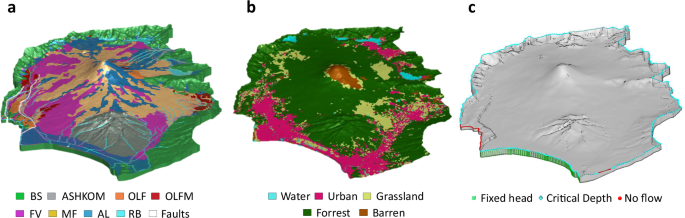
Set up for the integrated hydrogeological model of Mt. Fuji catchment (Japan); (a) Elemental zones in the porous medium domain, corresponding to the different hydrofacies in Table 1, as well as the lake and riverbeds (RB) and fault elements, corresponding to the lake and river beds, resp. to the fault zone; (b) Elemental zones for the overland flow domain, corresponding to the categories in Table 3; (c) Model boundary conditions: blue diamonds represent the critical depth boundary conditions for the surface domain in the Suruga Bay area, on the river outflows and on the catchment contours. The Fuji River Termination (SW) and Kise River effluent (SE) are set to no-flow boundary conditions (red spheres). The green boxes represent the fixed head for the subsurface domain in the Suruga bay area, and to the river elevation in the North and East outlets (not visible from this point of view). For the lateral subsurface boundaries for which no other boundary conditions are indicated, as well as for the base of the model, no flow conditions were imposed (not shown).
The hydraulic properties assigned to each hydrofacies are summarized in Table 1, with the exception of the hydraulic conductivity of BS and ASHKOM. As part of the sensitivity analyses (described hereafter), depth-dependent hydraulic conductivity was implemented for these hydrofacies following the approach proposed in the literature117, which characterizes permeability as an exponentially decreasing function with depth. This method is particularly suited for volcanic basement formations, where high near-surface permeability due to fracturing decreases due to increasing overburden stress and mineralization. Given the similarity of the BS and ASHKOM layers to the volcanic units of the Oregon Cascades, the following equation was applied for depths z < 1.5 km:
$$K\left(z\right)={K}_{s}\cdot {e}^{-z/d}$$
(1)
Where K(z) [m d−1] is the hydraulic conductivity at depth z [m], Ks is the near-surface hydraulic conductivity [m d−1], and d is the characteristic depth of permeability decrease [m]. Using the values Ks = 4.3 m d−1 and d = 75 m, this formulation ensures a realistic permeability decrease with depth while maintaining a finite value at the surface. At depths greater than 2,000 m, the calculated values from this approach converge with those reported in Table 1, ensuring consistency with previously established parameterizations for deep basement formations. The chosen parameters are consistent with observed permeability structures in volcanic basement rocks117. In the model, this was implemented by first calculating the coordinates of each element’s centroid, determining its depth, and then applying Eq. 1.
In addition to the hydrofacies described in Table 1, to better represent surface–subsurface interactions, the elements beneath lakes and rivers (i.e., lakebed and riverbed sediments, referred to as RB in Fig. 4) in the uppermost model layer were assigned a reduced hydraulic permeability (K = 10−8 m s−1). This reflects the presence of fine-grained, low-permeability lacustrine sediments as observed in Lake Yamanaka and Lake Motosu118,119 and addresses the fact that riverbed sediments generally exhibit a lower conductivity than the surrounding alluvial sediments due to deposition of fines and the subsequent formation of a colmation layer102,120.
Assignment of hydraulic properties for the fault zone
In volcanic watershed models, faults can significantly disrupt the continuity of hydrofacies layers. Depending on their composition and structural characteristics, faults may act either as barriers (e.g., due to low-permeability fault gouge or clay-rich lithologies) or as preferential flow conduits. Stratovolcanoes are typically located in tectonic constellations such as active subduction zones. In such locations, incorporating 3D fault structures is essential for preserving the geological integrity of hydrofacies distributions and ensuring the reliability of surface–subsurface hydrological simulations.
At Mt. Fuji, the influence of the Iriyamase segment within the FKFZ on groundwater dynamics—specifically on total hydraulic head distribution and salinity—has been investigated using conceptual and numerical models70, which indicate that this fault zone exhibits high permeability. Based on these findings, elements adjacent to the modeled fault traces, extending through the entire vertical profile, were assigned elevated hydraulic conductivity values (K = 10−3 m s−1; see Fig. 4).
While HGS supports discrete fracture network (DFN) representations using dual- or multiple-permeability domain121, an implicit fault-zone parameterization was chosen for computational efficiency. This choice prioritizes scalability and model performance while still honouring the key hydrogeological role of major fault structures.
Sensitivity analysis of subsurface hydraulic properties
Initial simulations with spatially uniform K values and no sediment layers resulted in widespread, unrealistic water retention patterns, including widespread surface ponding in topographically rugged areas and overly persistent saturation. Subsequent incorporation of depth-dependent K values117 improved subsurface flow behavior but caused simulated lakes to drain fully. To address this, lakebed sediment information118,119 was incorporated, introducing a low-permeability layer that restored realistic lake representation. Finally, reduced-permeability riverbed sediments were included to improve surface-subsurface dynamics102,120,122. These iterative refinements improved model realism and numerical stability, highlighting the importance of depth-dependent K values and surface waterbed resistance in establishing a robust base configuration for future use and calibration.
Assignment of hydraulic properties for the surface domain
The surface domain is parametrized using the LULC dataset. The original LULC dataset considered 14 distinct land-use types, which for the purpose of this ISSHM modeling exercise were aggregated into five broader categories based on their influence on surface hydrological processes such as infiltration, runoff, and evapotranspiration, using QGIS.
The first category, Water and Wetlands, includes water bodies and wetlands. Impervious Urban Areas consist of built-up areas, solar panel installations, and greenhouses, and are characterized by low infiltration rates and high surface runoff. The Grassland and Agriculture category encompasses paddy fields, croplands, and grasslands, which exhibit moderate infiltration. Forests, including deciduous broad-leaved, deciduous needle-leaved, evergreen broad-leaved, evergreen needle-leaved, and bamboo forests, have high infiltration capacities and are expected to play a significant role in canopy interception and evapotranspiration. Lastly, the Barren Areas category, represented by bare ground, is characterized by low infiltration and high runoff potential. The parameters for each zone are summarized in Table 3. In HGS, the zones were implemented by reading the dominant class directly from the aggregated raster file and are shown in Fig. 4b.
Table 3 Surface flow domain properties for the different land-use categories.Manning’s roughness coefficients are based on established values from the literature (refs. 130,131).
Surface–subsurface hydrological interactions in HGS are defined to be computed using the dual node approach121. A uniform exchange length lexch [m] coefficient of 0.1 m was considered for the entire model domain, striking a balance between ensuring smooth exchange fluxes between the surface and subsurface domains and guaranteeing numerical stability.
Definition of hydrologic boundary conditions
For the subsurface domain, boundary conditions (BCs) were assigned as follows: Dirichlet boundary conditions (constant head) corresponding to 710 m asl and 260 m asl were defined along the lateral model boundaries of the Katsura and Ayuzawa river valleys located in the North and East of the catchment. In the South all along the subsurface interface to Suruga Bay, a constant head of 0 m asl (freshwater equivalent) was employed, allowing for both submarine groundwater discharge and drainage through the Fuji and Kano rivers. A freshwater head was used instead of a seawater-equivalent head because the system is SGD-dominated56, salinity effects are negligible on the scale of the hydraulic gradients, and density-driven flow was not simulated. No-flow boundaries were assigned to the remaining lateral and bottom subsurface boundaries of the subsurface domain (Fig. 4c) as the model domain is based on the topographic catchment, and no data are available to justify deeper or transboundary flows.
For the surface domain, a critical-depth boundary condition was applied along all boundaries, allowing water to exit the model freely. Two specific sections of the lateral model boundary require distinct treatments:
1.
Fuji River Termination (SW Border) – The Fuji River, originating within the catchment, follows the catchment’s southwestern edge before discharging into Suruga Bay. It is fed by both the Fuji catchment and contributions from the mountain ranges on the western side
2.
Kise River Effluent (SE Border) – A short section of the Kise River briefly exits the catchment before re-entering. Before re-entering, it is joined by the Kano River, which originates in the Izu Peninsula.
By treating these sections as no-flow boundaries, all the water contributed to these rivers by Mt. Fuji catchment could be retained within the model domain until the rivers reached their proper outlets. As this underestimates the total discharge of these river systems at their outlets, river discharge observations for the Fuji and Kano rivers into the Suruga Bay area cannot be directly used for model parametrization. This treatment also pragmatically accounts for the FKFZ along the southwestern boundary, which connects to the Fuji River catchment but lies outside the scope of this model.
Evapotranspiration was not explicitly simulated, both to reduce computational complexity and because the primary focus of this study is on structural model development, rather than detailed surface energy or water balance processes. Actual evapotranspiration, which amounts to approximately 1000 mm yr−¹ (ref. 47), was, however, considered by subtracting it from the total average of 2500 mm yr−¹ of precipitation that falls on Mt. Fuji catchment each year50 and by applying a uniform rainfall rate of 1600 mm yr−¹ throughout the entire catchment.
Definition of hydrologic initial conditions, model spin-up and model run parameters
For the initial model spin-up, contour lines of the mean hydraulic heads in Mt. Fuji catchment available through the Water Environment Map of Mt. Fuji platform123 are digitized in QGIS, rasterized, and then used as input to define the initial head distribution in the subsurface domain in HGS. For the surface domain, an initial water depth of 0.00 m is used (i.e., default parametrization). Once the hydraulic heads have reached the quasi-steady state (approx. 10,000 yrs of simulation), the resulting hydraulic head distributions in the subsurface and on the surface are iteratively used as initial conditions for subsequent simulations with more refined parameterizations.
Simulations are controlled using a Newton-Raphson solver and an adaptive time-stepping scheme, starting from an initial time step of approximately 1 microsecond with a maximum timestep of 100 days for a total simulation duration of 3,000 yrs. This is sufficiently long to reach a new quasi-steady-state in all hydrogeologic formations for simulations started using the quasi-steady state heads of the spin-up model. The Newton absolute and Newton residual convergence criteria of HGS are set to 10−2 m.
Using this setup, a simulation of Mt. Fuji catchment of 3,000 yrs with constant boundary conditions takes about 24 h to reach a new quasi-steady-state using 6 CPU in parallel on a regular desktop with an Intel i9-12900K processor and 32 Gb of DDR5 RAM. Export of model results
The 3D ISSHM model geometries, numerical mesh, hydraulic parameters, boundary conditions, and model outputs were exported from HGS in Tecplot and Paraview-compatible format for post-processing, visualization, and technical validation. These files are available in the associated repository91.
AloJapan.com