

As the validation of homogeneity for the combined time series of the sea ice dates, we first investigated three standard metrics: level shift, trend shift, and standard deviation (STD) shift from the previous window to the following window. A large value (both positive and negative) at a connection point indicates a caution that the reconstruction of time series might not be robust. Note that natural variabilities and shifts on several time scales are also included, for example, as influenced by the Pacific Decadal Oscillation (PDO)26. Thus, the shift values at the connection points are compared with other large values that are known as natural variabilities; if the value at a connection point is as large as or larger than those for the natural shifts, the homogeneity at the connection point is concerned. The window width was set to 15 years (including the target year) to reduce the influence of the decadal variabilities (e.g., PDO). Hence, for the shift metrices in 2000, for example, values for 1986–2000 and 2000–2014 were compared. Level denotes the mean value (day of year) during the window, trend denotes the linear trend, and STD is calculated from differences from the level value.
For the FD_sight time series (Fig. 5a), relatively large level shifts around 1919 and 1939 are perceived before the connection point (1945–1946), but level shifts at similar magnitudes are also seen after that (in the 1980s and the 1990s). Trend shifts are relatively large in magnitude recently with a negative peak around 1989 and a positive peak around 2003. STD shifts are almost within the range from −5 to 5 days. Thus, no peak was detected at the connection point in terms of these validation metrices, supporting the homogeneity of the time series.
Fig. 5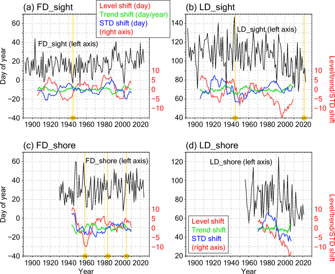
Validation of homogeneity for the sea ice dates. (a) FD_sight. (b) LD_sight. (c) FD_shore. (d) LD_shore. Black lines denote the sea ice dates in day of year (accumulative days from 1 January; e.g. 32 for 1 February and −2 for 29 December in the previous year). Validation metrices, level shift (unit in day; right axis), trend shift (day/year), and standard deviation (STD) shift (day) from the previous 15 years to the following 15 years are plotted by red, green, and blue lines, respectively. Since FD_shore and LD_shore were not defined in 1989 because drift ice did not connect to land-fast ice, the metrices were calculated without these data. Data connection years (Table 2) are indicated by yellow vertical lines and circles in (a–c).
For the LD_sight time series (Fig. 5b), the connection points are 1945–1946 and 2021–2022. STD shifts are relatively large (negative) around 1946 but not so larger than other large STD shifts seen in the 1920s and the 1980s; hence, we can consider that artificial shifts do not occur in the former connection point. In terms of the latter connection point, the extended data period of two years is not enough and further validation should be conducted when the data are accumulated in the future, although the time series do not seem unnatural and the final parts of the validation metrices are not so large.
For the FD_shore time series (Fig. 5c), the published JMA records cover the data from 1959 and the data during 1930–1958 was extended in this study. Thus, large (negative) level shifts are seen around the connection point. In addition, relatively large (positive) level and STD shifts are seen around 1945–1946. These variations in level shift seem to result from relatively large FD_shore values (late dates) in the late 1940s and the 1950s. On the large shifts around 1945–1946, although we could not find description of the change in the observation method (definition), changes associated with the JMA establishment might affect the measurements, while there is a possibility that the large shifts reflect the natural decadal variations. We will discuss these shifts in the FD_shore time series later with the drift ice amount data. Other than this possible connection (1945–1946) and the definition changes of FD_shore as described in Method section, changes in the shapes of the breakwaters (as indicated by solid lines toward the lights in Fig. 2b) and in the shadow regions (dashed line in Fig. 2b; e.g. in 2015) due to house building might affect the observation homogeneity near the shore (both FD_shore and LD_shore). Thus, we should note that the homogeneity of the FD_shore time series might be weaker at the connection points than the other sea ice dates. Nevertheless, we retained the extended FD_shore time series since it might reflect an aspect of the local climate and be useful for future studies accompanied by other datasets.
For the LD_shore time series (Fig. 5d), the official JMA data are not extended. Negative level shifts are remarkable after the 1980s similar to LD_sight. These can be physically understood as these sea ice last dates have recently shifted to earlier dates as a result of regional warming27. The STD shifts are relatively large around 1980. Again, we could not access whether these STD shifts are detecting artificial connection or not and retained the time series as the original JMA data.
The daily time series of total sea ice amount (Fig. 6) has already been used in climate studies11,12. Although the data in 2021 were added in this study, the data were obtained at the Abashiri Local Meteorological Office with the same manner. In this study, we investigated (1) ice amount-weighted central day (“weighted center”) from the first positive day to the last positive day of the year and (2) accumulated SIC that is sum of the daily SIC values (fraction of 0–1) during the sea ice period, for evaluating the time series. The weighted center time series (Fig. 6b) are mostly within the range 40–70 (day of year), suggesting that the mature stage of total ice generally takes place in February–early March. Although negative level and STD shifts are seen after the 1990s, the magnitudes are much smaller than the metrices for the accumulated SIC (Fig. 6c). In the accumulated SIC time series, remarkable reduction can be seen around 1989, which is reflected in a negative peak of the level shift in the same year and the change of the sign of the trend shift; also the trend shift takes negative values afterward. The above reduction would be related to the abrupt reduction of sea ice over the Sea of Okhotsk in 1989 as described in the previous study28.
Fig. 6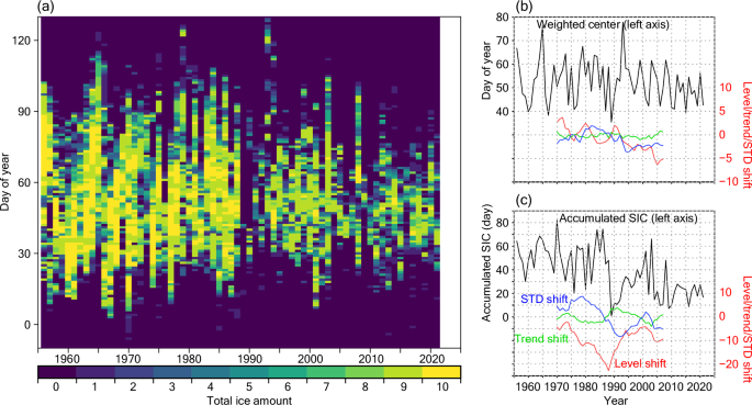
Statistics of total ice amount. (a) Daily total ice amount time series in 10th quantile. x-axis denotes year and y-axis denote day of year. (b,c) Weighted center (b) and accumulated SIC (c) of the total ice for each year (black line). Validation metrices, level shift (unit in day; right axis), trend shift (day/year), and standard deviation (STD) shift (day) from the previous 15 years to the following 15 years are plotted by red, green, and blue lines, respectively.
For the drift ice amount (Fig. 7), the variations of the validation metrices are similar to those for the total ice amount (Fig. 6); the impacts of the great reduction in 198928 are remarkable in the SIC and the accumulated SIC time series (Fig. 7a,c, respectively). In addition, the longer time series (from 1930) allows us to detect another negative peak of the level shift around the late 1940s. The large accumulated SIC values before the middle of 1940s are consistent with the stably small FD_shore values (early dates) in the same period with small STDs (Fig. 5c). Note that the drift ice amount measurements would be less affected by the near-shore constructions than the FD_shore measurements. Thus, the above consistency lends support to the applicability of the FD_shore time series even in the early years (before 1945). Actually, the previous study19 linked the relatively large sea ice amounts in these early years to increasing trend of the surface temperature. This dataset would be of value as a diagnostic tool of the North Pacific climate variability and global warming.
Fig. 7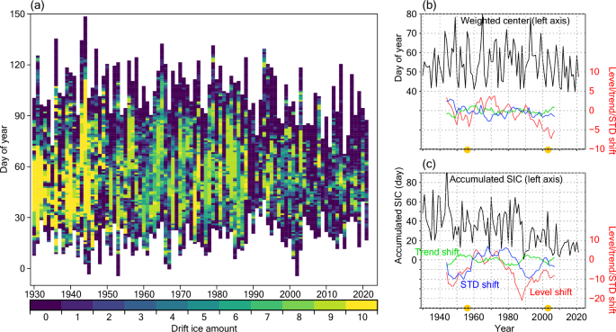
Statistics of drift ice amount. Same as Fig. 6 but for drift ice. For (a), only data from FD_sight till LD_sight are plotted for each year. Data connection years (Table 2) are indicated by yellow circles in (b,c). Note that drift ice amount values can be zero even on the FD_sight and LD_sight dates since these dates are often determined based on additional observations (other than at 9:00 JST).
Cumulative deviation from the mean (CDM) approach has also been used for tests of time series homogeneity29. We focus on the validation for the relatively long time series, FD_sight and LD_sight. As shown in Fig. 8, the CDM values (green lines; normalized by standard deviation) become as large as 20 for both FD_sight and LD_sight, indicating that the homogeneity is not valid. However, the peak values appear around 1980s, whereas the values at the connection points (vertical yellow lines; Table 2) are relatively small; hence, the discontinuities are attributable to the natural shift as described above28. Actually, the CDM peaks are much smaller for the time series before (1892–1975; blue lines) and after (1996–2025; red lines) the discontinuous period due to the natural variation. In these time series (blue and red), the CDM values are rather small in the connection points, suggesting that discontinuities due to the connection of the time series are smaller than the natural variability.
Fig. 8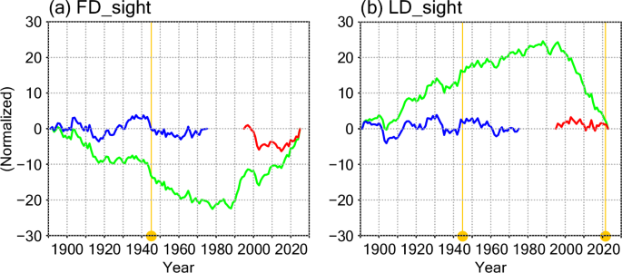
Cumulative deviation from the mean (CDM) time series. (a) FD_sight. (b) LD_sight. Green lines denote the CDM values for the whole observation periods: 1892–2025 in (a) and 1892–2023 in (b). Blue and red lines denote the CDM values for the period before 1975 and after 1996, respectively. Data connection years (Table 2) are indicated by yellow vertical lines and circles.
Table 2 Connection points of the different data sources to create long time records.
In summary for this validation section, unnatural variations associated with discontinuity of the observation method were not clearly detected. The remarkable variations (i.e. discontinuity) of the total and drift ice amounts in 1989 are consistent with the previous study.
AloJapan.com